ECE 205 Notes

First Order Linear Differential Equations

$y^{\prime }+p(x)y=f(x)$$y'+p(x)y = f(x)$

Variation of Parameters Method

Find a integrating factor $\mu (x)$$\mu(x)$ that makes $\mu (x)y^{\prime }+\mu (x)p(x)y=(\mu (x)y{)}^{\prime }=f(x)\mu (x)$$\mu(x)y' + \mu(x)p(x)y = (\mu(x)y)' = f(x)\mu(x)$

Then $\mu (x)y=\int f(x)\mu (x)dx$$\mu(x)y = \int f(x)\mu(x)dx$

$\mu (x)p(x)={\mu }^{\prime }(x)⟹\mu (x)=e^{\int p(x)dx}\text{(Separating variables)}$$\mu(x)p(x) = \mu'(x) \implies \mu(x) = e^{\int p(x)dx} \text{(Separating variables)}$

Homegeneous

$y^{\prime }+p(x)y=0$$y' + p(x)y = 0$

$y(x)=C{e}^{-\int p(x)dx}$$y(x) = Ce^{-\int p(x)dx}$

Non-Homegeneous

$y^{\prime }+p(x)y=f(x)$$y'+p(x)y = f(x)$

Use variation of parameters Method

Existence and Uniqueness of solution Theorem (?)

$y_1$$y_1$ is any nontrival solution to non-homogeneous equation

General solution:

$y(x)=y_1(x)(c+\int \frac{f(x)}{y_1(x)}dx)$$y(x) = y_1(x)(c + \int\frac{f(x)}{y_1(x)}dx)$

Unique solution for $y(x_0)=y_0$$y(x_0) = y_0$:

$y(x)=y_1(x)(\frac{y_0}{y_1(0)}+{\int }_{x_0}^x\frac{f(t)}{y_1(t)}dt)$$y(x) = y_1(x)(\frac{y_0}{y_1(0)} + \int^x_{x_0}\frac{f(t)}{y_1(t)}dt)$

Separable Equations (Separting Variables Method)

A differential equation is said to be separable if it can be written as $h(y)y^{\prime }=g(x)$$h(y)y' = g(x)$

$h(y)dy=g(x)dx$$h(y)dy = g(x)dx$

$\int h(y)dy=\int g(x)dx$$\int h(y)dy = \int g(x)dx$

$H(y)=G(x)+C$$H(y) = G(x) + C$

Implicit Solutions

A relation $G(x,y)=0$$G(x,y) = 0$, is said to be an implicit solution on the interval $I$$I$ if it defines one or more explicit solution on $I$$I$.

Constant Solution

$y^{\prime }=0$$y' = 0$, 注意不要漏掉这些解

Difference between linear and non-linear equations

对于linear equation，可以选取任意的$y_0$$y_0$，总可以通过选择合适的常量C使general solution变成IVP $y(x_0)=y_0$$y(x_0) = y_0$的解($x_0\in (a,b)$$x_0 \in (a,b)$

对于non-linear equation，对于不同的$y_0$$y_0$，interval of valiadity 会变化($x_0$$x_0$ 的范围随$y_0$$y_0$变化)

Exact Equations

The differential equation form $M(x,y)dx+N(x,y)dy=0$$M(x,y)dx + N(x,y)dy = 0$ is said to be exact in a rectangle $R$$R$ if there is a function $F(x,y)$$F(x,y)$ such that: $F_x=M$$F_x = M$ and $F_y=N$$F_y = N$, for all $(x,y)\in R$$(x,y) \in R$

Check for existance of F

$M(x,y)dx+N(x,y)dy=0$$M(x,y)dx + N(x,y)dy = 0$ is an exact equation in R if and only if $M_y=N_x$$M_y = N_x$ for all $(x,y)\in R$$(x,y) \in R$

$M_y=F_{xy}=F_{yx}=N_x$$M_y = F_{xy} = F_{yx} = N_x$

Integrating factor:

When ${\mu }_y=0$$\mu_y = 0$

$-{\mu }_{x}N=(N_x-M_y)\mu$$-\mu_x N = (N_x - M_y)\mu$

${\mu }^{\prime }=\frac{M_y-N_x}{N}\mu$$\mu' =\frac{M_y-N_x}{N}\mu$

$\mu (x)=e^{\int \frac{M_y-N_x}{N}dx}$$\mu(x) = e^{\int \frac{M_y-N_x}{N}dx}$

When ${\mu }_x=0$$\mu_x = 0$

${\mu }_{y}M=(N_x-M_y)\mu$$\mu_y M = (N_x - M_y) \mu$

${\mu }^{\prime }=\frac{N_x-M_y}{M}\mu$$\mu' = \frac{N_x-M_y}{M}\mu$

$\mu (y)=e^{\int \frac{N_x-M_y}{M}dx}$$\mu (y) = e^{\int \frac{N_x - M_y}{M}dx}$

Then, use either of them to find F

$F=\int F_{x}dx+g(y)=\int \mu (x)M(x,y)dx+g(y)$$F = \int F_x dx + g(y) = \int \mu(x)M(x,y) dx + g(y)$

$F_y=(\int \mu (x)M(x,y)dx{)}_y+g^{\prime }(y)=\mu (x)N(x,y)$$F_y = (\int \mu(x)M(x,y) dx)_y + g'(y) = \mu(x)N(x,y)$

The solution is $F=C$$F=C$

Second Order Linear Differential Equations

$y^{″}+p(x)y^{\prime }+q(x)y=f(x)$$y'' + p(x)y' + q(x)y = f(x)$

Homogeneous Linear Equations

$y^{″}+p(x)y^{\prime }+q(x)y=0$$y'' + p(x)y' + q(x)y = 0$

If $y_1$$y_1$ and $y_2$$y_2$ are solutions of the homogeneous equation, then any linear combination $y=c_1{y}_1+c_2{y}_2$$y =c_1y_1 + c_2y_2$ is also a solution on $(a,b)$$(a,b)$

The set $\{y_1,y_2\}$$\{y_1, y_2\}$ is a fundemental set if $\{y_1,y_2\}$$\{y_1, y_2\}$ is linearly independent on $(a,b)$$(a,b)$

Wronskian

$y_1,y_2$$y_1,y_2$ are linearly independent on $(a,b)$$(a,b)$ if and only if $W$$W$ has no zeros on $(a,b)$$(a,b)$

Abel's Formula

因此，W要么都不为0，要么都是0

Constant Coefficients Homegeneous Equations

$a{y}^{″}+b{y}^{\prime }+cy=0$$ay'' + by' + cy = 0$

Let $y(x)=e^{rx}$$y(x) = e^{rx}$

$a{r}^2{e}^{rx}+br{e}^{rx}+c{e}^{rx}=e^{rx}(a{r}^2+br+c)=0$$ar^2e^{rx} + bre^{rx} + ce^{rx} = e^{rx}(ar^2+br+c) = 0$

Characteristic Equation: $a{r}^2+br+c=0$$ar^2 + br + c = 0$

Solution: $y=e^{rx}$$y = e^{rx}$, where $r=\frac{-b\pm \sqrt{b^2-4ac}}{2a}$$r = \frac{-b\pm \sqrt{b^2-4ac}}{2a}$

Distinct Real Roots

$y(x)=c_1{e}^{rx}+c_2{e}^{rx}$$y(x) = c_1e^{rx} + c_2e^{rx}$

Repeated Real Root

$y_1(x)=e^{rx}$$y_1(x) = e^{rx}$

Assume $y_2(x)=u(x)e^{rx}$$y_2(x) = u(x)e^{rx}$

$y_2^{\prime }(x)=u^{\prime }(x)e^{rx}+u(x)r{e}^{rx}$$y_2'(x) = u'(x)e^{rx} + u(x)re^{rx}$

$y_2^{″}(x)=u^{″}(x)e^{rx}+u^{\prime }(x)r{e}^{rx}+u^{\prime }(x)r{e}^{rx}+u(x)r^2{e}^{rx}$$y_2''(x) = u''(x)e^{rx} + u'(x)re^{rx} + u'(x)re^{rx} + u(x)r^2e^{rx}$

$a{u}^{″}(x)e^{rx}+(2ar+b)u^{\prime }(x)e^{rx}+(a{r}^2+br+c)u(x)e^{rx}=0$$au''(x)e^{rx} + (2ar+b)u'(x)e^{rx}+(ar^2 + br + c)u(x)e^{rx} = 0$

当选择r为Repeated Real Root时，$a{r}^2+br+c=0$$ar^2 + br + c = 0$, $2ar+b=\frac{d(a{r}^2+br+c)}{dr}=0$$2ar + b = \frac{d(ar^2 + br + c)}{dr} = 0$ (二次函数的顶点)

因此$a{u}^{″}(x)e^{rx}=0⟹u^{\prime }(x)=k_1⟹u(x)=k_{1}x+k_0$$au''(x)e^{rx} = 0 \implies u'(x) = k_1 \implies u(x) = k_1x + k_0$

Choose $k1=1,k_0=0⟹y_2(x)=x{e}^{rx}$$k1 = 1, k_0 = 0 \implies y_2(x) = xe^{rx}$

$y(x)=c_1{e}^{rx}+c_{2}x{e}^{rx}$$y(x) = c_1e^{rx} + c_2xe^{rx}$

Complex Conjugate Roots

Euler's formula: $e^{i\theta }=cos\theta +isin\theta$$e^{i\theta} = cos\theta + isin\theta$

Non-Homogeneous Linear Equations

The Method of Undetermined Coefficients

$a{y}^{″}+b{y}^{\prime }+cy=C{x}^m{e}^{rx}$$ay'' + by' + cy = Cx^me^{rx}$

$y_p(x)=x^s(A_m{x}^m+\cdots +A_{1}x+A_0)e^{rx}$$y_p(x) = x^s(A_mx^m + \cdots + A_1x + A_0)e^{rx}$

s = 0: r is not a root to charastic equation

s = 1: r is simple root to charastic equation

s = 2: r is double root to charastic equation

$a{y}^{″}+b{y}^{\prime }+cy=C{x}^m{e}^{\alpha x}cos(\beta x)$$ay'' + by' + cy = Cx^me^{\alpha x} cos (\beta x)$ (or $sin(\beta x)$$sin(\beta x)$ )

$y_p(x)=x^s(A_m{x}^m+\cdots +A_{1}x+A_0)e^{\alpha x}cos(\beta x)+x^s(B_m{x}^m+\cdots +B_{1}x+B_0)e^{\alpha x}sin(\beta x)$$y_p(x) = x^s(A_mx^m + \cdots + A_1x + A_0)e^{\alpha x}cos(\beta x) + x^s(B_mx^m + \cdots + B_1x + B_0)e^{\alpha x}sin(\beta x)$

s = 0: $\alpha +i\beta$$\alpha + i \beta$ is not a root to charastic equation

s = 1: $\alpha +i\beta$$\alpha + i \beta$ is a root to charastic equation

The Superposition Principle

If $y_1$$y_1$ is a solution to $a{y}^{″}+b{y}^{\prime }+cy=f_1(x)$$ay'' + by' + cy = f_1(x)$, $y_2$$y_2$ is a solution to $a{y}^{″}+b{y}^{\prime }+cy=f_2(x)$$ay'' + by' + cy = f_2(x)$

Then, $y=k_1{y}_1+k_2{y}_2$$y = k_1 y_1 + k_2y_2$ is a solution to the differential equation: $a{y}^{″}+b{y}^{\prime }+cy=k_1{f}_1(x)+k_2{f}_2(x)$$ay'' + by' + cy = k_1f_1(x) + k_2f_2(x)$

For any non-homogeneous linear equation $a{y}^{″}+b{y}^{\prime }+cy=f(x)$$ay'' + by' + cy = f(x)$, the solution is given by the sum of Complementary Solution and Particular Solution

$y(x)=c_1{y}_1(x)+c_2{y}_2(x)+y_p(x)$$y(x) = c_1y_1(x) + c_2y_2(x) + y_p(x)$

参考线性代数中的nullspace和particular solution

Variation of parameters

$a{y}^{″}+b{y}^{\prime }+cy=f(x)$$ay'' + by' + cy = f(x)$

$y_h(x)=C_1{y}_1(x)+C_2{y}_2(x)$$y_h(x) = C_1y_1(x) + C_2y_2(x)$

Instead of constants, let them be functions

$y_p(x)=v_1{y}_1+v_2{y}_2$$y_p(x) = v_1y_1 + v_2y_2$

为了简化运算，令$v_1^{\prime }{y}_1+v_2^{\prime }{y}_2=0$$v_1'y_1 + v_2'y_2 = 0$

$y_p^{\prime }(x)=v_1^{\prime }{y}_1+v_1{y}_1^{\prime }+v_2^{\prime }{y}_2+v_2{y}_2^{\prime }=v_1{y}_1^{\prime }+v_2{y}_2^{\prime }$$y_p'(x) = v_1'y_1 + v_1y_1' + v_2'y_2 + v_2y_2' = v_1y_1' + v_2y_2'$

$y_p^{″}(x)=v_1^{\prime }{y}_1^{\prime }+v_1{y}_1^{″}+v_2^{\prime }{y}_2^{\prime }+v_2{y}_2^{″}=v_1^{\prime }{y}_1^{\prime }+v_1{y}_1^{″}+v_2^{\prime }{y}_2^{\prime }+v_2{y}_2^{″}$$y_p''(x) = v_1'y_1' + v_1y_1'' + v_2'y_2' + v_2y_2'' = v_1'y_1' + v_1y_1'' +v_2'y_2' + v_2y_2''$

$v_1(a{y}_1^{″}+b{y}_1^{\prime }+c{y}_1)+v_2(a{y}_2^{″}+b{y}_2^{\prime }+c{y}_2)+a(v_1^{\prime }{y}_1^{\prime }+v_2^{\prime }{y}_2^{\prime })=f(x)$$v_1(ay_1'' + by_1' + cy_1) + v_2(ay_2'' + by_2' + cy_2) + a(v_1'y_1' + v_2'y_2') = f(x)$

因为$y_1,y_2$$y_1, y_2$ 为Homogeneous equation solution, $a{y}_1^{″}+b{y}_1^{\prime }+c{y}_1=a{y}_2^{″}+b{y}_2^{\prime }+c{y}_2=0$$ay_1'' + by_1' + cy_1 = ay_2'' + by_2' + cy_2 = 0$

$a(v_1^{\prime }{y}_1^{\prime }+v_2^{\prime }{y}_2^{\prime })=f(x)$$a(v_1'y_1' + v_2'y_2') = f(x)$

在带上之前的假设$v_1^{\prime }{y}_1+v_2^{\prime }{y}_2=0$$v_1'y_1 + v_2'y_2 = 0$

$v_2^{\prime }(y_2^{\prime }{y}_1-y_2{y}_1^{\prime })=y_{1}f(x)/a$$v_2' (y_2'y_1 - y_2y_1') = y_1f(x)/a$

Subsititue back

Note that $W=y_1{y}_2^{\prime }+y_1^{\prime }{y}_2$$W = y_1y_2' + y_1'y_2$

$v_1=\int \frac{-y_{2}f(x)}{aW}dx$$v_1 = \int \frac{-y_2f(x)}{aW}dx$

$v_2=\int \frac{y_{1}f(x)}{aW}dx$$v_2 = \int \frac{y_1f(x)}{aW}dx$

这个积分，若令常数项C=0，则为Particular solution $y_p(x)$$y_p(x)$

令常数项分别等于$C_1,C_2$$C_1, C_2$，则$y(x)=v_1{y}_1+v_2{y}_2$$y(x) = v_1y_1 + v_2y_2$ （积分的常数项变成了general solution）

Application: Spring problems

$m{u}^{″}+\gamma u^{\prime }+ku=F(t)$$mu'' + \gamma u' + ku = F(t)$

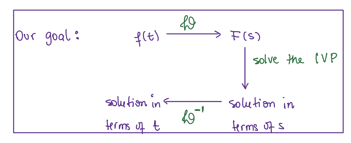
Laplace Transform

Integral Transforms

Useful tool for solving linear differential equations. An integral transform is a relation of the form $F(s)={\int }_0^{\mathrm{\infty }}k(s,t)f(t)dt$$F(s) = \int_0^{\infty} k(s,t)f(t)dt$, where $k(s,t)$$k(s,t)$ is a given function called kernel of transformation

T-domain IVP --transform--> S-domain IVP --solve--> S-domain solution --inverse transform--> T-domain solution

Laplace Transform

$F(s)={\int }_0^{\mathrm{\infty }}{e}^{-st}f(t)dt$$F(s) = \int_0^{\infty} e^{-st} f(t)dt$

Notation: $\mathcal{L}\{f(t)\}=F(s)$$\mathscr{L}\{f(t)\} = F(s)$

The laplace transform replaces linear constant coefficients D.E. in the t-domain by simpler algebraic equation in the s-domain

Properties of Laplace transform

[Theorem] Let $f_1,f_2$$f_1,f_2$ be functions whose Laplace transfroms exist for $s>\alpha$$s > \alpha$, and let $c_1,c_2$$c_1, c_2$ be constants, then for $s>\alpha$$s > \alpha$

$\mathcal{L}\{c_1{f}_1+c_2{f}_2\}=c_1\mathcal{L}\{f_1\}+c_2\mathcal{L}\{f_2\}$$\mathscr{L}\{c_1f_1 + c_2f_2\} = c_1\mathscr{L} \{f_1\} + c_2 \mathscr{L}\{f_2\}$

拉普拉斯变换是线性的

[Def] A function f(t) is said to be piecewie continuous on a finite interval $[a,b]$$[a,b]$ if f(t) is continuous at every point in $[a,b]$$[a,b]$, except possible for a finite number of points which f(t) has a jump discontinuity. A function f(t) is said to be piecewise continuous on $[0,\mathrm{\infty })$$[0, \infty)$ if f(t) is piecewise continuous on $[0,T]$$[0, T]$ for all $T>0$$T > 0$

[Def] A function f(t) is said to be exponential order $\alpha$$\alpha$ if there exist positive constants T and M such that $|f(t)|\le M{e}^{\alpha t}$$|f(t)| \leq Me^{\alpha t}$

[Theorem] If f(t) is piecewise continuous $[0,\mathrm{\infty })$$[0, \infty)$ and of exponential order $\alpha$$\alpha$, then $\mathcal{L}\{f\}(s)$$\mathscr{L}\{f\}(s)$ exists for $s>\alpha$$s > \alpha$

[例] f(t) = 1/t 不存在拉普拉斯变换

[Theorem] If the Laplace transform $\mathcal{L}\{f(t)\}(s)=F(s)$$\mathscr{L}\{f(t)\}(s) = F(s)$ exists for $s>\alpha$$s > \alpha$, then $\mathcal{L}\{e^{\alpha t}f(t)\}(s)=F(s-a),s>\alpha +a$$\mathscr{L}\{e^{\alpha t} f(t)\}(s) = F(s-a), s > \alpha + a$

乘一个指数倍相当于在s域上平移

[例] $\mathcal{L}\{sin(bt)\}=\frac{b}{s^2+b^2}$$\mathscr{L}\{sin(bt)\} = \frac{b}{s^2 + b^2}$, $\mathcal{L}\{e^{at}sin(bt)\}=\frac{b}{(s-a{)}^2+b^2}$$\mathscr{L}\{e^{at}sin(bt)\} = \frac{b}{(s-a)^2 + b^2}$

The Inverse Laplace Transform

[Def] Given a function F(s), if there is a function f(t) that is continuous on $[0,\mathrm{\infty })$$[0, \infty)$ and satisfies $\mathcal{L}\{f\}=F$$\mathscr{L}\{f\} = F$, then we say f(t) is the inverse Laplace Transform of F(s) and employ $f={\mathcal{L}}^{-1}\{F\}$$f = \mathscr{L}^{-1}\{F\}$

[Theorem] ${\mathcal{L}}^{-1}\{c_1{F}_1+c_2{F}_2\}=c_1{\mathcal{L}}^{-1}\{F_1\}+c_2{\mathcal{L}}^1\{F_2\}$$\mathscr{L}^{-1}\{c_1F_1 + c_2F_2\} = c_1\mathscr{L}^{-1} \{F_1\} + c_2 \mathscr{L}^{1}\{F_2\}$

拉普拉斯逆变换也是线性的

Partial Function Decomposition

For non-repeated linear factors

$Q(s)=(s-r_1)(s-r_2)\cdots (s-r_n),r_i\in \mathbb{R}$$Q(s) = (s-r_1)(s-r_2) \cdots (s-r_n), r_i \in \mathbb{R}$, then $\frac{P(s)}{Q(s)}=\frac{A_1}{s-r_1}+\frac{A_2}{s-r_2}+\cdots +\frac{A_n}{s-r_n}$$\frac{P(s)}{Q(s)} = \frac{A_1}{s-r_1} + \frac{A_2}{s-r_2} + \cdots + \frac{A_n}{s-r_n}$

For repeated linear factors

$Q(s)=(s-r{)}^m(s-r_1)(s-r_2)\cdots (s-r_n)$$Q(s) = (s-r)^m(s-r_1)(s-r_2)\cdots(s-r_n)$, then $\frac{P(s)}{Q(s)}=\frac{A_1}{s-r}+\frac{A_2}{(s-r{)}^2}+\cdots +\frac{A_m}{(s-r{)}^m}+\cdots$$\frac{P(s)}{Q(s)} = \frac{A_1}{s-r} + \frac{A_2}{(s-r)^2} + \cdots + \frac{A_m}{(s-r)^m} + \cdots$

一般思路：进行partial fraction decomposition后，对每一个项进行逆变换

Solution of initial value problem

[Theorem] Let f(t) be continuous on $[0,\mathrm{\infty })$$[0, \infty)$ and f'(t) be piecewise continuous on $[0,\mathrm{\infty })$$[0, \infty)$ with both exponential order $\alpha$$\alpha$. Then, for $s>\alpha$$s > \alpha$, $\mathcal{L}\{f^{\prime }\}(s)=s\mathcal{L}\{f\}(s)-f(0)$$\mathscr{L}\{f'\}(s) = s\mathscr{L}\{f\}(s) - f(0)$

Generalize之后：

[Theorem] Let $f(t),f^{\prime }(t),...,f^{(n-1)}(t)$$f(t), f'(t), ..., f^{(n-1)}(t)$ be continuous on $[0,\mathrm{\infty })$$[0, \infty)$ and $f^{(n)}(t)$$f^{(n)}(t)$ be piecewise continuous on $[0,\mathrm{\infty })$$[0, \infty)$ with all these functions exponential order $\alpha$$\alpha$. Then, for $s>\alpha$$s > \alpha$, $\mathcal{L}\{f^{(n)}\}(s)=s^n\mathcal{L}\{f\}(s)-s^{n-1}f(0)-s^{n-2}{f}^{\prime }(0)-...-f^{(n-1)}(0)$$\mathscr{L}\{f^{(n)}\}(s) = s^n\mathscr{L}\{f\}(s) - s^{n-1}f(0) - s^{n-2}f'(0) - ... - f^{(n-1)}(0)$

Laplace Transform of Piecewise Continuous Functions

Unit Step function

[Theorem] Let $g$$g$ be defined on $[0,\mathrm{\infty })$$[0, \infty)$. Suppose $a\ge 0$$a \geq 0$ and $\mathcal{L}\{g(t+a)\}$$\mathscr{L}\{g(t+a)\}$ exists for $s>s_0$$s > s_0$. Then $\mathcal{L}\{u(t-a)g(t)\}$$\mathscr{L}\{u(t-a)g(t)\}$ exists for $s>s_0$$s > s_0$, and $\mathcal{L}\{u(t-a)g(t)\}=e^{-sa}\mathcal{L}\{g(t+a)\}$$\mathscr{L}\{u(t-a)g(t)\} = e^{-sa}\mathscr{L}\{g(t+a)\}$

同理，$\mathcal{L}\{u(t-a)g(t-a)\}=e^{-sa}\mathcal{L}\{g(t)\}$$\mathscr{L}\{u(t-a)g(t-a)\} = e^{-sa}\mathscr{L}\{g(t)\}$

Constant coefficient equations

如果要有解必须满足

1. $y(0)=k_0,y^{\prime }(0)=k_1$$y(0) = k_0, y'(0) = k_1$

2. $y,y^{\prime }$$y, y'$ 在$[0,\mathrm{\infty })$$[0,\infty)$上连续

3. $y^{″}$$y''$在每个开区间都是有定义的，同时在每个间断点都有左右极限

Convolution

[Def] The convolution $f\ast g$$f*g$ of two functions f and g is defined by

$(f\ast g)(t)={\int }_0^{t}f(\tau )g(t-\tau )d\tau$$(f*g)(t) = \int_0^t f(\tau)g(t-\tau)d\tau$

Properties

$f\ast g=g\ast f$$f*g = g*f$ $f\ast (g+h)=f\ast g+f\ast h$$f*(g+h) = f*g + f*h$ $(f\ast g)\ast h=f\ast (g\ast h)$$(f*g)*h = f*(g*h)$ $f\ast 0=0$$f*0 = 0$

[Theorem] If$\mathcal{L}\{f\}=F$$\mathscr{L}\{f\} = F$, and $\mathcal{L}\{g\}=G$$\mathscr{L}\{g\} = G$, then $\mathcal{L}\{f\ast g\}=FG$$\mathscr{L}\{f*g\} = FG$

Constant Coefficient Equations with Impulses

Dirac Delta furction $\delta$$\delta$:

$\mathcal{L}\{\delta (t)\}=1$$\mathscr{L}\{\delta(t)\} = 1$

$\mathcal{L}\{\delta (t-t_0)\}=e^{-s{t}_0}$$\mathscr{L}\{\delta(t-t_0)\} = e^{-st_0}$

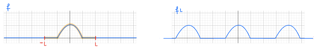
Fourier Series

$cos(\frac{m\pi x}{L})$$cos(\frac{m\pi x}{L})$ 与 $sin(\frac{m\pi x}{L})$$sin(\frac{m\pi x}{L})$的特性

Common Period: $T=2\pi /\omega =2L/m$$T = 2\pi / \omega = 2L/m$, 因此，f(x)的最大周期为2L

Orthogonality

类似线性代数，定义函数的inner product 为$(u,v)={\int }_{\alpha }^{\beta }u(t)v(t)dt$$(u,v) = \int_\alpha^\beta u(t)v(t)dt$

并且定义$u(t),v(t)$$u(t), v(t)$在interval $[\alpha ,\beta ]$$[\alpha, \beta]$上orthogonal 若 inner product = 0, a set of functions is said to be mutually orthogonal if each distinct pair of functions in the set is orthogonal

[Theorem] The functions $cos(\frac{m\pi x}{L}),sin(\frac{m\pi x}{L})$$cos(\frac{m\pi x}{L}), sin(\frac{m\pi x}{L})$, $m=1,2,...$$m = 1,2,...$ form a mutually orthogonal set on the interval $-L\le x\le L$$-L \leq x \leq L$

可以用积化和差公式证明，只有当同为sin或同为cos时，且m = n时，inner product = L, 否则= 0

奇偶函数积分性质: ${\int }_{-a}^a(odd)=0$$\int_{-a}^a (odd) = 0$, ${\int }_{-a}^a(even)={\int }_0^{2a}(even)$$\int_{-a}^a (even) = \int_0^{2a} (even)$

Computing Fourier Coefficients

$a_m=\frac{1}{L}{\int }_{-L}^{L}f(x)cos(\frac{m\pi x}{L})dx$$a_m = \frac{1}{L}\int_{-L}^L f(x) cos(\frac{m\pi x}{L})dx$

$b_m=\frac{1}{L}{\int }_{-L}^{L}f(x)sin(\frac{m\pi x}{L})dx$$b_m = \frac{1}{L}\int_{-L}^L f(x) sin(\frac{m\pi x}{L})dx$

利用的是orthogonality，乘上一个指定频率的三角函数后，由于orthogonality，只会得到f(x)中频率以及相位符合的那个分量的系数，其余的都互相垂直，积分为0

对于$a_0$$a_0$，直接对原式求积分

由于三角函数的一个完整周期的积分 = 0，因此

${\int }_{-L}^{L}f(x)dx={\int }_{-L}^L\frac{a_0}{2}dx⟹a_0=\frac{1}{L}{\int }_{-L}^{L}f(x)dx$$\int_{-L}^L f(x)dx = \int_{-L}^L\frac{a_0}{2} dx \implies a_0 = \frac{1}{L}\int_{-L}^L f(x)dx$

Initial-boundry value problem - The Heat Equation

PDE: $u_t=\beta u_{xx},0<x<L,t>0$$u_t = \beta u_{xx}, 0 < x < L, t > 0$

Boundry Conditions: $u(0,t)=u(L,t)=0$$u(0, t) = u(L,t) = 0$

Initial Condition(t = 0): $u(x,0)=f(x)$$u(x,0) = f(x)$

解法：

Separation of Variables, suppose $u(x,t)=X(x)T(t)$$u(x,t) = X(x)T(t)$

$u_t=\beta u_{xx}⟹X(x)T^{\prime }(t)=\beta X^{″}(x)T(t)$$u_t = \beta u_{xx} \implies X(x)T'(t) = \beta X''(x)T(t)$

$\frac{T^{\prime }(t)}{\beta T(t)}=\frac{X^{″}(x)}{X(x)}=-\lambda$$\frac{T'(t)}{\beta T(t)} = \frac{X''(x)}{X(x)} = -\lambda$

于是我们得到了两个ODE

$X^{″}(x)+\lambda X(x)=0$$X''(x) + \lambda X(x) = 0$

$T^{\prime }(t)+\lambda \beta T(t)=0$$T'(t) + \lambda \beta T(t) = 0$

我们现在考虑Boundry Conditions

$u(0,t)=X(0)T(t)=0$$u(0,t) = X(0)T(t) = 0$

$u(L,t)=X(L)T(t)=0$$u(L,t) = X(L)T(t) = 0$

$⟹(X(0)-X(L))T(t)=0$$\implies (X(0) - X(L))T(t) = 0$

$T\equiv 0$$T \equiv 0$ or $X(0)=X(L)$$X(0) = X(L)$

若T为0函数，则u(x,t)也为0函数，所以我们希望取$X(0)=X(L)=0$$X(0) = X(L) = 0$

把Boundry condition与ODE结合起来得到一个BVP - Boundry Value Problem

$X^{″}(x)+\lambda X(x)=0,X(0)=X(L)=0$$X''(x) + \lambda X(x) = 0, X(0) = X(L) = 0$

目的：For what values of $\lambda$$\lambda$, the BVP has non-trivial solutions?

Non-trivial solutions are called eignfunctions, the special values are called eigenvalues

假设$X(x)=e^{rx}$$X(x) = e^{rx}$，characteristic equation: $r^2+\lambda =0$$r^2 + \lambda = 0$，求解constant coefficient secondary linear DE

对不同$\lambda$$\lambda$ 取值分类讨论

$\lambda <0$$\lambda < 0$， Distinct Real roots

$X(x)=c_1{e}^{\sqrt{-\lambda }x}+c_2{e}^{-\sqrt{-\lambda }x}$$X(x) = c_1e^{\sqrt{-\lambda}x} + c_2e^{-\sqrt{-\lambda}x}$

$X(0)=c_1+c_2=0⟹X(L)=c_1{e}^{\sqrt{-\lambda }L}+c_2{e}^{-\sqrt{-\lambda }L}=c_1(e^{\sqrt{-\lambda }L}-e^{-\sqrt{-\lambda }L})=0$$X(0) = c_1 + c_2 = 0 \implies X(L) = c_1e^{\sqrt{-\lambda}L} + c_2e^{-\sqrt{-\lambda}L} = c_1(e^{\sqrt{-\lambda}L} - e^{-\sqrt{-\lambda}L}) = 0$

$⟹c_1=c_2=0⟹X\equiv 0,trivial$$\implies c_1 = c_2= 0 \implies X \equiv 0,trivial$

$\lambda =0$$\lambda = 0$, Repeated Real root

$X(x)=c_1+c_{2}x$$X(x) = c_1 + c_2x$

$X(0)=c_1=0⟹X(L)=c_{2}L=0⟹c_2=0$$X(0) = c_1 = 0 \implies X(L) = c_2L = 0 \implies c_2 = 0$

$⟹X\equiv 0,trivial$$\implies X \equiv 0, trivial$

$\lambda >0$$\lambda > 0$, Complex conjugate roots

$X(x)=c_{1}cos(\sqrt{\lambda }x)+c_{2}sin(\sqrt{\lambda }x)$$X(x) = c_1cos(\sqrt \lambda x) + c_2 sin(\sqrt \lambda x)$

$X(0)=c_1=0⟹X(L)=c_{2}sin(\sqrt{\lambda }L)=0$$X(0) = c_1 = 0 \implies X(L) = c_2sin(\sqrt \lambda L) = 0$

$c_2=0$$c_2 = 0$ or $\sin \left(\lambda L\right)=0$$\sin(\lambda L) = 0$, for non-trivial solutions, we want the latter

Eignvalue $sin(\sqrt{\lambda }L)=0⟹\sqrt{\lambda }L=n\pi ⟹\lambda =(\frac{n\pi }{L}{)}^2$$sin(\sqrt \lambda L) = 0 \implies \sqrt \lambda L = n\pi \implies \lambda = (\frac{n\pi}{L})^2$

$X(x)=c_{2}sin(\sqrt{\lambda }x)⟹X_n(x)=a_{n}sin(\frac{n\pi x}{L})$$X(x) = c_2sin(\sqrt \lambda x) \implies X_n(x) = a_n sin(\frac{n\pi x}{L})$

代入$T^{\prime }(t)+\beta \lambda T(t)=0$$T'(t) + \beta \lambda T(t) = 0$

$T^{\prime }(t)+\beta (\frac{n\pi }{L}{)}^{2}T(t)=0⟹T_n(t)=b_n{e}^{-\beta (\frac{n\pi }{L}{)}^{2}t}$$T'(t) + \beta (\frac{n\pi}{L})^2 T(t) = 0 \implies T_n(t) = b_n e^{-\beta (\frac{n\pi}{L})^2 t}$

$u_n(x,t)=X_n(x)T_n(t)=a_{n}sin(\frac{n\pi x}{L})b_n{e}^{-\beta (\frac{n\pi }{L}{)}^{2}t}$$u_n(x,t) = X_n(x)T_n(t) = a_n sin(\frac{n\pi x}{L}) b_n e^{-\beta (\frac{n\pi}{L})^2 t}$

$c_n=a_n{b}_n$$c_n = a_nb_n$

$u(x,t)={\mathrm{\Sigma }}_{n=1}^{\mathrm{\infty }}{c}_n{e}^{-\beta (\frac{n\pi }{L}{)}^{2}t}sin(\frac{n\pi x}{L})$$u(x,t) = \Sigma_{n=1}^{\infty} c_n e^{-\beta (\frac{n\pi}{L})^2 t} sin(\frac{n\pi x}{L})$

为什么要 求和？：对于任何满足要求的X(x)，都可以在任意的频率上有任意的系数同时满足ODE，可以理解为每个n代表着一个null space的一个basis vector，而求和则是linear combination

最后求solution，只需把$u(x,0)=f(x)$$u(x,0) = f(x)$代入后，计算每个n对应的$c_n$$c_n$

$u(x,0)={\mathrm{\Sigma }}_{n=1}^{\mathrm{\infty }}{c}_{n}sin(\frac{n\pi x}{L})$$u(x,0) = \Sigma_{n=1}^{\infty} c_n sin(\frac{n\pi x}{L})$

The wave equation

跟Heat equation 类似，但由于PDE两边都是双重导数，有略微差别

PDE: $u_{tt}={\alpha }^2{u}_{xx},0<x<L,t>0$$u_{tt} = \alpha ^2 u_{xx}, 0 < x < L, t > 0$

Boundry Conditions: $u(0,t)=u(L,t)=0,t\ge 0$$u(0,t) = u(L,t) = 0, t \geq 0$

Initial Conditions: $u(x,0)=f(x),u_t(x,0)=g(x)$$u(x,0) = f(x), u_t(x,0) = g(x)$

同样使用separation of variables, $u(x,t)=X(x)T(t)$$u(x,t) = X(x)T(t)$

$u_t=\beta u_{xx}⟹X(x)T^{″}(t)={\alpha }^2{X}^{″}(x)T(t)$$u_t = \beta u_{xx} \implies X(x)T''(t) = \alpha^2 X''(x)T(t)$

两个ODE:

$X^{″}(x)+\lambda X(x)=0$$X''(x) + \lambda X(x) = 0$

$T^{″}(t)+\lambda {\alpha }^{2}T(t)=0$$T''(t) + \lambda \alpha^2 T(t) = 0$

Boundry Condition 与上面Heat equation的相同，同时对于X的ODE也相同，因此eignvalue $\lambda =(\frac{n\pi }{L}{)}^2$$\lambda = (\frac{n\pi}{L})^2$

$X_n(x)=c_{n}sin(\frac{n\pi x}{L})$$X_n(x) = c_n sin(\frac{n\pi x}{L})$

$T^{″}(t)+(\frac{n\pi }{L}{)}^2{\alpha }^{2}T(t)=0$$T''(t) + (\frac{n\pi}{L})^2 \alpha^2 T(t) = 0$

characteristic equation: $r^2+(\frac{n\pi \alpha }{L}{)}^2=0$$r^2 + (\frac{n \pi \alpha}{L})^2 = 0$, complex conjugate roots

$T_n(t)=c_{n,1}cos[(\frac{n\pi \alpha }{L})t]+c_{n,2}sin[(\frac{n\pi \alpha }{L})t]$$T_n(t) = c_{n,1} cos[(\frac{n \pi \alpha}{L})t ] + c_{n,2} sin[(\frac{n \pi \alpha}{L})t]$

$u_n(x,t)=c_{n}sin(\frac{n\pi x}{L})[c_{n,1}cos[(\frac{n\pi \alpha }{L})t]+c_{n,2}sin[(\frac{n\pi \alpha }{L})t]]$$u_n(x,t) = c_n sin(\frac{n\pi x}{L}) [c_{n,1} cos[(\frac{n \pi \alpha}{L})t ] + c_{n,2} sin[(\frac{n \pi \alpha}{L})t]]$

$a_n=c_n{c}_{n,1},b_n=c_n{c}_{n,2}$$a_n = c_n c_{n,1}, b_n = c_n c_{n,2}$

$u(x,t)={\mathrm{\Sigma }}_{n=1}^{\mathrm{\infty }}[a_{n}cos[(\frac{n\pi \alpha }{L})t]+b_{n}sin[(\frac{n\pi \alpha }{L})t]]sin(\frac{n\pi x}{L})$$u(x,t) = \Sigma_{n=1}^\infty [a_n cos[(\frac{n \pi \alpha}{L})t ] + b_n sin[(\frac{n \pi \alpha}{L})t]]sin(\frac{n\pi x}{L})$

然后代入两个Initial Condition即可得到Solution

$u(x,0)={\mathrm{\Sigma }}_{n=1}^{\mathrm{\infty }}{a}_{n}sin(\frac{n\pi x}{L})$$u(x,0) = \Sigma_{n=1}^\infty a_nsin(\frac{n\pi x}{L})$

$u_t(x,t)={\mathrm{\Sigma }}_{n=1}^{\mathrm{\infty }}[-a_n(\frac{n\pi \alpha }{L})sin[(\frac{n\pi \alpha }{L})t]+b_n(\frac{n\pi \alpha }{L})cos[(\frac{n\pi \alpha }{L})t]]sin(\frac{n\pi x}{L})$$u_t(x,t) = \Sigma_{n=1}^\infty [-a_n (\frac{n \pi \alpha}{L}) sin[(\frac{n \pi \alpha}{L})t ] + b_n (\frac{n \pi \alpha}{L})cos[(\frac{n \pi \alpha}{L})t]]sin(\frac{n\pi x}{L})$

$u_t(x,0)={\mathrm{\Sigma }}_{n=1}^{\mathrm{\infty }}{b}_n(\frac{n\pi \alpha }{L})sin(\frac{n\pi x}{L})={\mathrm{\Sigma }}_{n=1}^{\mathrm{\infty }}{B}_{n}sin(\frac{n\pi x}{L})$$u_t(x,0) = \Sigma_{n=1}^\infty b_n (\frac{n \pi \alpha}{L})sin(\frac{n\pi x}{L}) = \Sigma_{n=1}^\infty B_nsin(\frac{n\pi x}{L})$

Fourier Sin and Cos Functions

从上面两个问题的解可以看出来，这种PDE求解后都需要将f(x)变为只含有sin的series

2L-period extensions

令2L = T

Fourier sine series

For odd function $f_o(x)$$f_o(x)$

$f_o(x)={\mathrm{\Sigma }}_{n=1}^{\mathrm{\infty }}{b}_{n}sin(\frac{n\pi x}{L})$$f_o(x) = \Sigma_{n=1}^{\infty}b_n sin(\frac{n\pi x}{L})$

$b_n=\frac{1}{L}{\int }_{-L}^L{f}_o(x)sin(\frac{n\pi x}{L})dx=\frac{2}{L}{\int }_0^{L}f(x)sin(\frac{n\pi x}{L})dx$$b_n = \frac{1}{L} \int_{-L}^L f_o(x) sin(\frac{n\pi x}{L})dx = \frac{2}{L}\int_0^L f(x) sin(\frac{n\pi x}{L})dx$

由于剩下两个项都是偶函数，不能出现在odd function的transform里，所以$a_0=a_n=0$$a_0 = a_n = 0$

(odd)(odd) = (even) (Even)(even) = (even) (odd)(even) = (odd)

${\int }_{-a}^a(odd)=0$$\int_{-a}^a (odd) = 0$ ${\int }_{-a}^a(even)=2{\int }_0^a(even)$$\int_{-a}^a (even) = 2\int_0^{a} (even)$

Fourier cosine series

$f_e(x)=\frac{a_0}{2}+{\mathrm{\Sigma }}_{n=1}^{\mathrm{\infty }}{a}_{n}cos(\frac{n\pi x}{L})$$f_e(x) = \frac{a_0}{2} + \Sigma_{n=1}^{\infty}a_ncos(\frac{n\pi x}{L})$

$a_n=\frac{1}{L}{\int }_{-L}^L{f}_e(x)cos(\frac{n\pi x}{L})dx=\frac{2}{L}{\int }_0^{L}f(x)cos(\frac{n\pi x}{L})dx$$a_n = \frac{1}{L} \int_{-L}^L f_e(x) cos(\frac{n\pi x}{L})dx = \frac{2}{L}\int_0^L f(x) cos(\frac{n\pi x}{L})dx$

$a_0$$a_0$ 只要代入n = 0, $a_0=\frac{2}{L}{\int }_0^{L}f(x)dx$$a_0 = \frac{2}{L}\int_0^L f(x)dx$

Convergence of Fourier Series

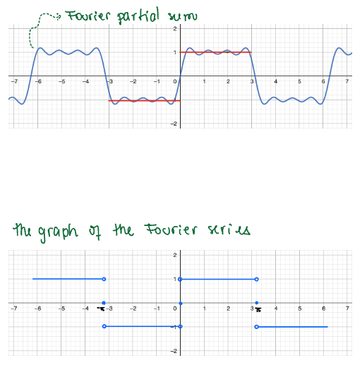
[Theorem - pointwise convergence] If $f,f^{\prime }$$f, f'$ are piecewise continuous on $[-L,L]$$[-L, L]$, then for any x in $(-L,L)$$(-L, L)$

$\frac{a_0}{2}+{\mathrm{\Sigma }}_{m=1}^{\mathrm{\infty }}[a_{m}cos(\frac{m\pi x}{L})+b_{m}sin(\frac{m\pi x}{L})]=\frac{1}{2}[f(x^{+})+f(x^{-})]$$\frac{a_0}{2} + \Sigma_{m = 1}^{\infty}[ a_m cos(\frac{m\pi x}{L}) + b_m sin(\frac{m\pi x}{L}) ] = \frac{1}{2}[f(x^+) + f(x^-)]$

For $x=\pm L$$x = \pm L$, the series converges to $\frac{1}{2}[f(L^{+})+f(L^{-})]$$\frac{1}{2}[f(L^+) + f(L^-)]$

如果一个函数有间断点，那么fourier series在间断点会converge到中间点

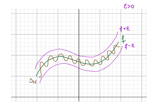
[Theorem] Let $f$$f$ be a continuous function on $(-\mathrm{\infty },\mathrm{\infty })$$(-\infty, \infty)$, and periodic of period 2L. $f^{\prime }$$f'$ is piecewise continuous on $[-L,L]$$[-L, L]$, then the Fourier series for $f$$f$ converges uniformly to $f$$f$ on $[-L,L]$$[-L, L]$ and hence on any interval.

Converge uniformly 的意思:

只要N足够大，converge的误差越小

[Proposition - Weierstrass m-test] If $|a_n(x)|\le M_n$$|a_n(x)| \leq M_n$ for all $x\in [a,b]$$x \in [a,b]$, and ${\mathrm{\Sigma }}_{n=1}^{\mathrm{\infty }}{M}_n$$\Sigma_{n=1}^{\infty} M_n$ converges , then ${\mathrm{\Sigma }}_{n=1}^{\mathrm{\infty }}{a}_n(x)$$\Sigma_{n=1}^{\infty} a_n(x)$ converges uniformly on $[a,b]$$[a,b]$, with sum $f(x)$$f(x)$

A test for proving that a series of functions converges uniformly on an interval

有点像infinite series的comparison test?

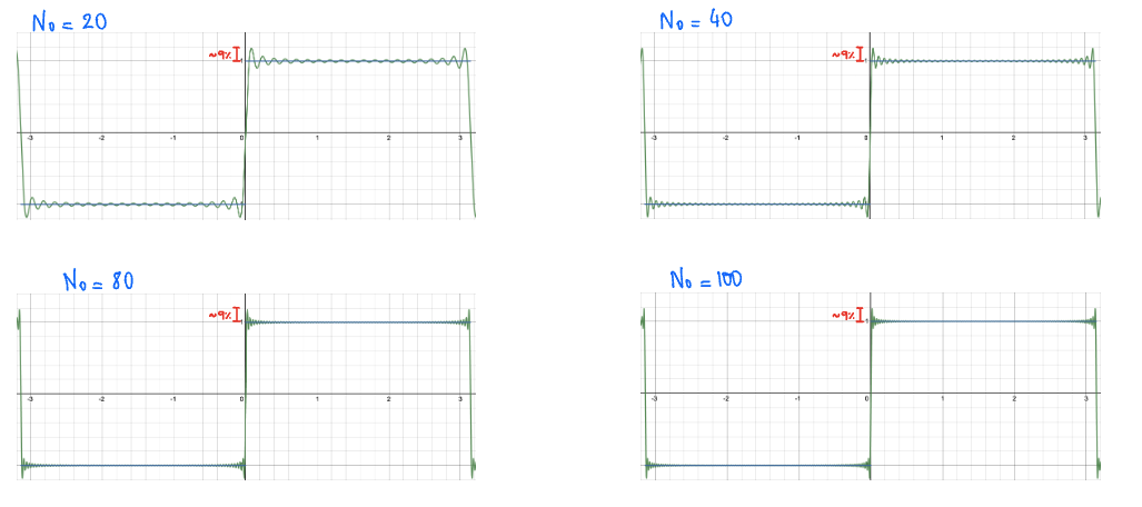
Gibbs Phenomenon

Near poinst of discontinuity of $f$$f$, the Fourier series may overshoot by approximately 9% of the jump regardless of N.

Differentiation and Integration of Fourier Series

对于不连续的函数，求导后会出现无穷大的值，导致fourier series 无法converge，因此做出如下限制条件

[Theorem] Let $f$$f$ be continuous on $(-\mathrm{\infty },\mathrm{\infty })$$(-\infty, \infty)$ and 2L-periodic. Let $f^{\prime }(x),f^{″}(x)$$f'(x), f''(x)$ be piecewise continuous on $[-L,L]$$[-L,L]$. Then, the fourier series for f(x) by termwise differentiation.