Finding the Minimum Inserts to Form a Palindrome
Given a string of length n (n<=10), characters can be inserted at any position to make it a palindrome. For example, “banana” can become a palindrome by inserting a ‘b’ at the rightmost position, so f(“banana”) = 1.
Analysis
The main challenge of this problem is finding the recursive approach. At first, I fell into a pit, trying to find the longest palindrome substring inside and then categorizing the two sides for discussion. Later, I found that this approach would lead to a complex and hard-to-implement algorithm.
Just when things seemed desperate, a “banana” suddenly inspired me. If we only look at the characters at the beginning and end each time, continue looking inside if they are the same, or insert the left side to the right side if they are different, and then do the same operation on the remaining inside - for example, in “abacca,” only adding ‘ba’ to the right side is needed.
But there is a problem - inserting characters on the right side is not always the best solution. For example, in “abacc,” the best solution is to add ‘cc’ on the left side, not ‘aba’ on the right side.
The Magic of “min” in Recursion
To solve this problem, one just needs to try both methods, and at this point, it is essential not to think globally but to focus on small problems.
The principle of this recursive function is to give a string “a{str}b,” where {str} is a string of any length, and ‘a’ and ‘b’ represent individual characters.
First, Consider the Case of a==b
Assuming X is a palindrome, then aXb is directly a palindrome, so no characters need to be inserted, return 0.
If X is not a palindrome, we can make it a palindrome by inserting f(X) characters, so in this case, f(aXb) equals f(X).
Case of a!=b
In this case, you can insert an ‘a’ on the right side, making it become f(aXba) which reverts back to the previous case, hence f(aXba) = f(Xb).
Or insert a ‘b’ on the left side, making it f(baXb) = f(aX).
What’s the use of f(aXba) and f(baXb)?
aXba is obtained by inserting a character in aXb, and baXb is the same, so f(aXb) = f(aXba) + 1, f(aXb) = f(baXb) + 1.
However, f(aXba) and f(baXb) are not necessarily the same. Since we are looking for the minimum amount, we just need to take the minimum of the two using min().
f(aXb) = min( f(aXba) + f(baXb) ) + 1 = min( f(Xb) + f(aX) ) + 1.
With that, we have successfully broken down a big problem into smaller ones, and now we can write the recursive solution.
But before diving into recursion, let’s handle the base cases first. Actually, there are only two base cases - one is when X is an empty string, and the other is when X has only one character (len(X) == 0, len(X) == 1). Both cases cannot form aXb. However, these cases themselves can be considered palindromes, so simply return 0.
Conclusion: The hardest part of this problem has ended
With just three lines of code, the recursive function can be written.
fn insert_pal_rec<T: std::cmp::PartialEq>(arr: &[T], start: usize, end: usize) -> usize{
    if end <= start { return 0; }
    if arr[start] == arr[end]{ return insert_pal_rec(&arr, start+1, end-1); }
    else{ return std::cmp::min(insert_pal_rec(&arr, start+1, end), insert_pal_rec(&arr, start, end-1)) + 1; }
}
This code can solve the problem, but there is still room for more optimization. The optimization part is the main motivation behind writing this blog post. So, if you are interested, you can continue reading for more.
High alert ahead, completely understanding the content requires knowledge of big O notation. However, if you just want to grasp the ideas and feel the charm of the algorithm, not having this knowledge doesn’t matter much. Don’t dwell too long on parts you haven’t understood.
[Side Note] How to Pass the Return Value? Thought Process of Recursive Calls
While studying my classmate’s code, I noticed someone passing an additional parameter ret during recursion to record the return value, like this:
import math
def process(str, ret):
    if base_case: return ret
    return process(str[1:-1], ret) if str[0] == str[-1] \
    else math.min(process(str[1:], ret+1), process(str[:-1], ret+1))
To explore which approach is better, I deliberately learned assembly language and looked at the compiled code, referring to this article “How to Pass the Return Value in Recursion? - Let’s Analyze Your Assembly Code!”
The Code Is Short, but How Efficient Is It?
Upon careful analysis of this code, it is evident that the time complexity is O(2^n^), and the space complexity is O(n).
Time: In the worst-case scenario, each character of
strneeds to be tried for adding to the left and right, meaning there are two possibilities for each character. During recursion, only two variables are passed, so it’s of constant size. The worst-case recursion depth is n-1 times because each time a character is reduced until there is only one left. If a newstrclone is passed during recursion, then the memory usage for passing values at each step becomes O(n), making the overall complexity O(n^2^).
Exponential time complexity is daunting. Now it’s clear why the limit n<=10 is set - even with the Rust code I wrote, this method wouldn’t work for a string of length n=30.
Why Is It So Slow? - Repeating the Same Work Many Times
Suppose we want to find the minimum insertions for the string “kcabad.” We can visualize this graph:
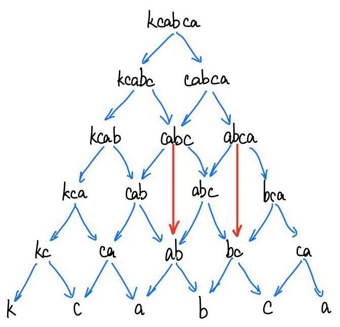
We can see that both f(kcabc) and f(cabca) require the value of f(cabc), which leads to f(cabc) being executed twice. f(ab) is even worse, as it needs to be called four times. However, it’s clear that the result returned by f(cabc) is not influenced by previous choices; it exhibits “optimal substructure.”
Hence, we have an insight: if we can cache the return values of the function, each function will be executed only once, saving significant time. By doing so, we can achieve an algorithm with a time complexity of O(n^2^) - this idea of caching is the essence of dynamic programming.
Memoization Index - Trading Space for Time
Upon deeper analysis, we realize that the previous recursion involved passing three values: the string, the starting position of the string, and the ending position of the string. The string remains constant throughout the recursion, which means that F() is a function dependent only on the start and end positions.
By slightly modifying the previous recursion and using a two-dimensional matrix to store all results, we can significantly boost the speed.
fn insert_pal_map<T: std::cmp::PartialEq>(arr: &[T]) -> usize{
    let mut map: Vec<Vec<Option<usize>>> = vec![vec![None; arr.len()]; arr.len()]; //initialize 2D array
    return process_with_map(&arr, 0, arr.len()-1, &mut map);
}
The time complexity becomes O(n^2^), and the space complexity becomes O(n^2^) (note that the space complexity due to recursion remains O(n), but focusing only on the highest-order term).
Organizing Thoughts - Strict Tabular Structure Steps In
Looking back at this tree diagram:
We recognize that the original problem can be seen as finding the shortest distance from top to bottom of this tree.
When two characters are equal, it’s like taking a shortcut on this road, skipping a layer. Therefore, the more shortcuts a path takes, the fewer characters are inserted.
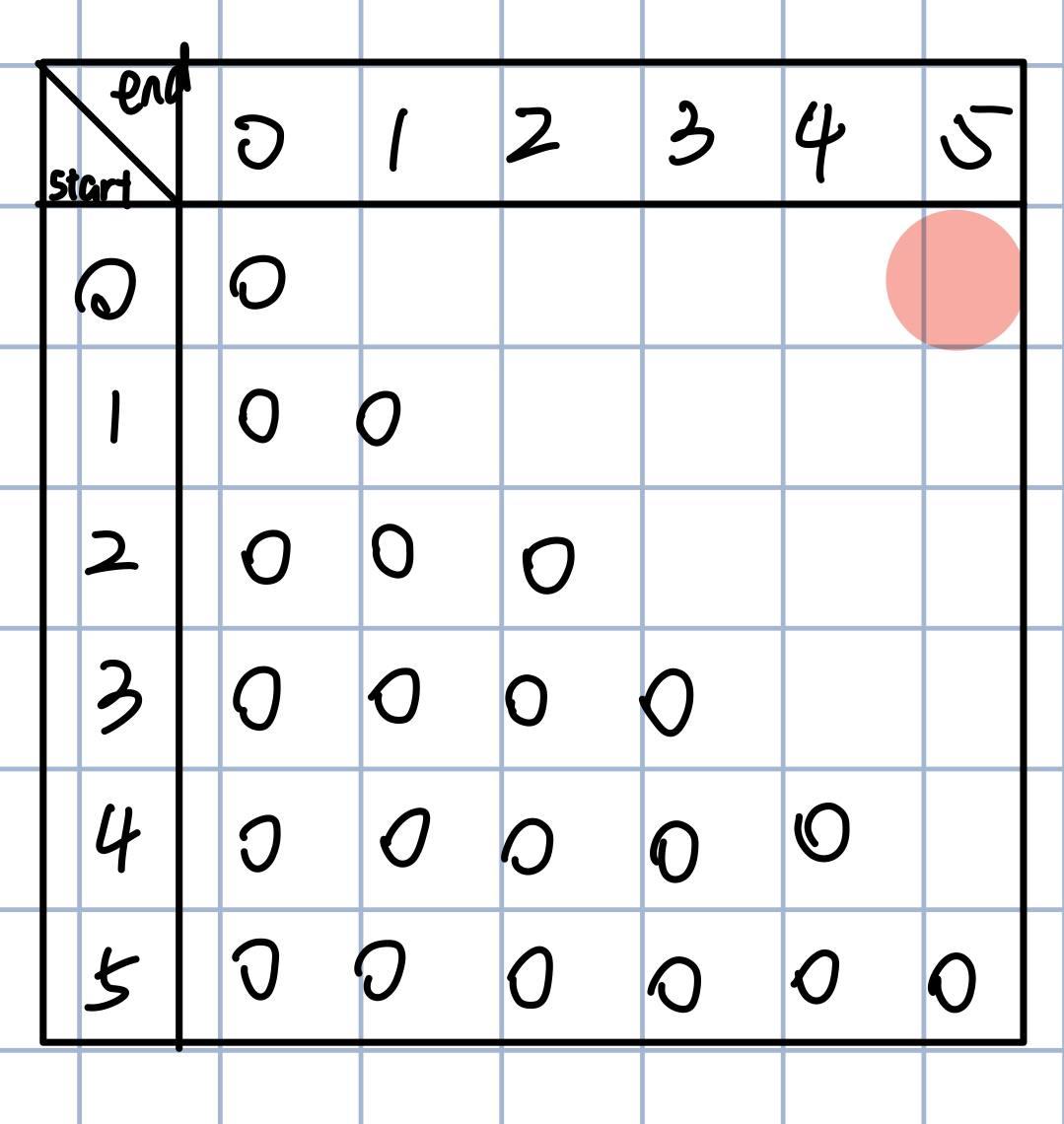
Now, if we analyze the last row, it precisely reflects each character of the original string. I had a bold idea - what if we start from the bottom and stack layer by layer, avoiding recursion, to find the final value?
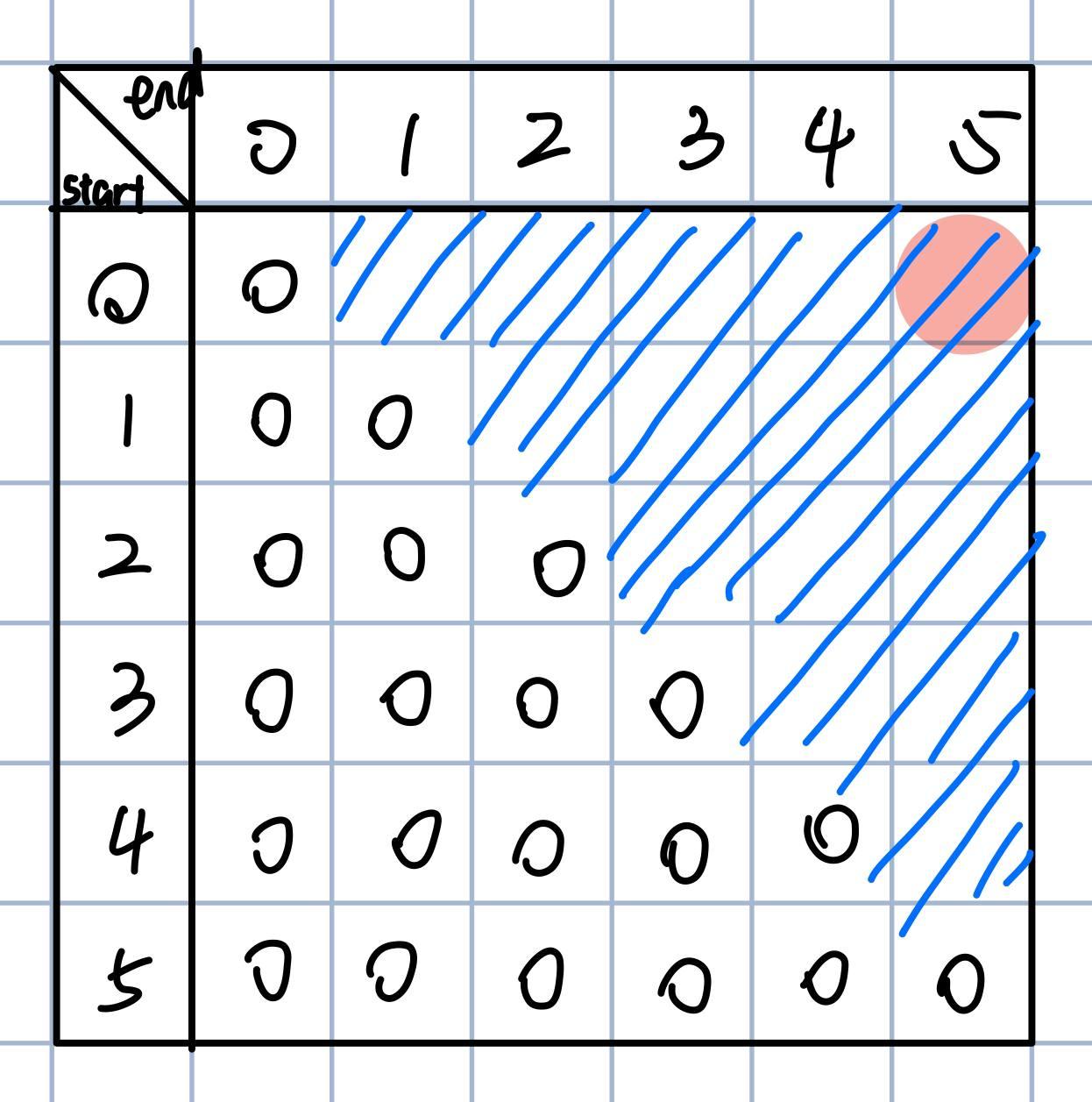
By setting up a matrix and filling it step by step, we aim to find the minimum insertions for “kcabca”:
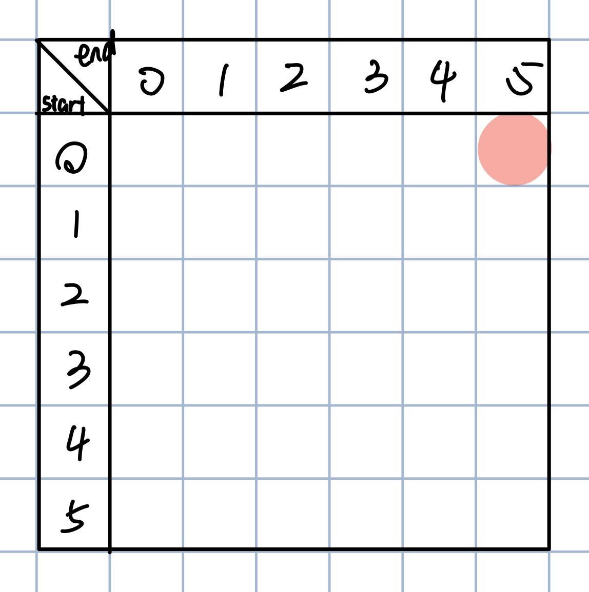
Each row represents a starting position, and each column represents an ending position. We aim for the position with start=0, end=5 (top right corner), so we need to fill in the rest based on the rules we observed earlier.
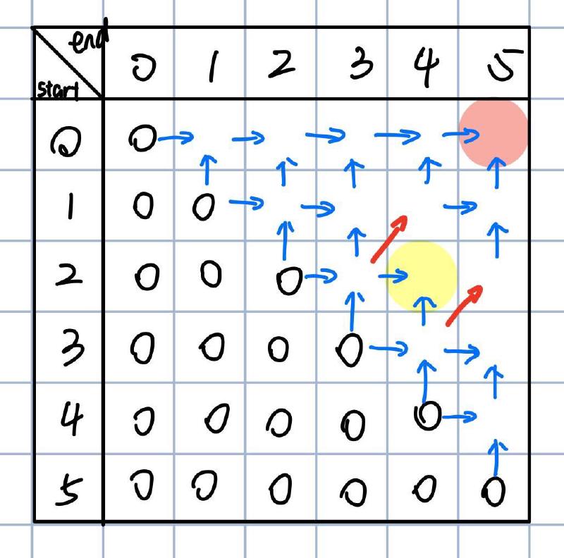
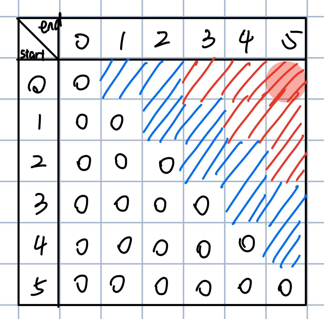
Following the recursion logic of checking character equality, we apply this step to the unfilled grid as well - marking it in red if the characters match:
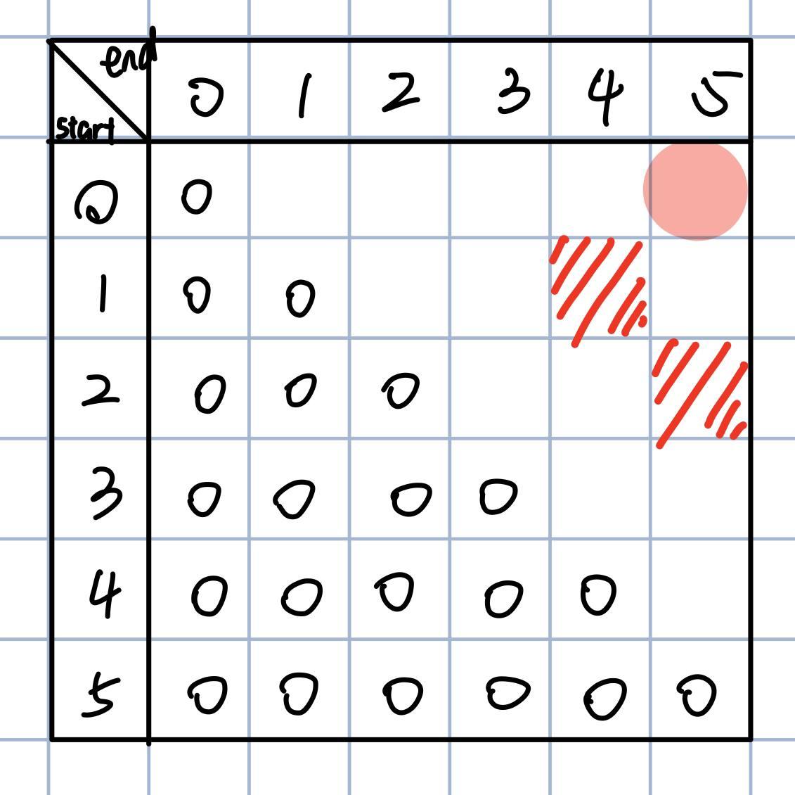
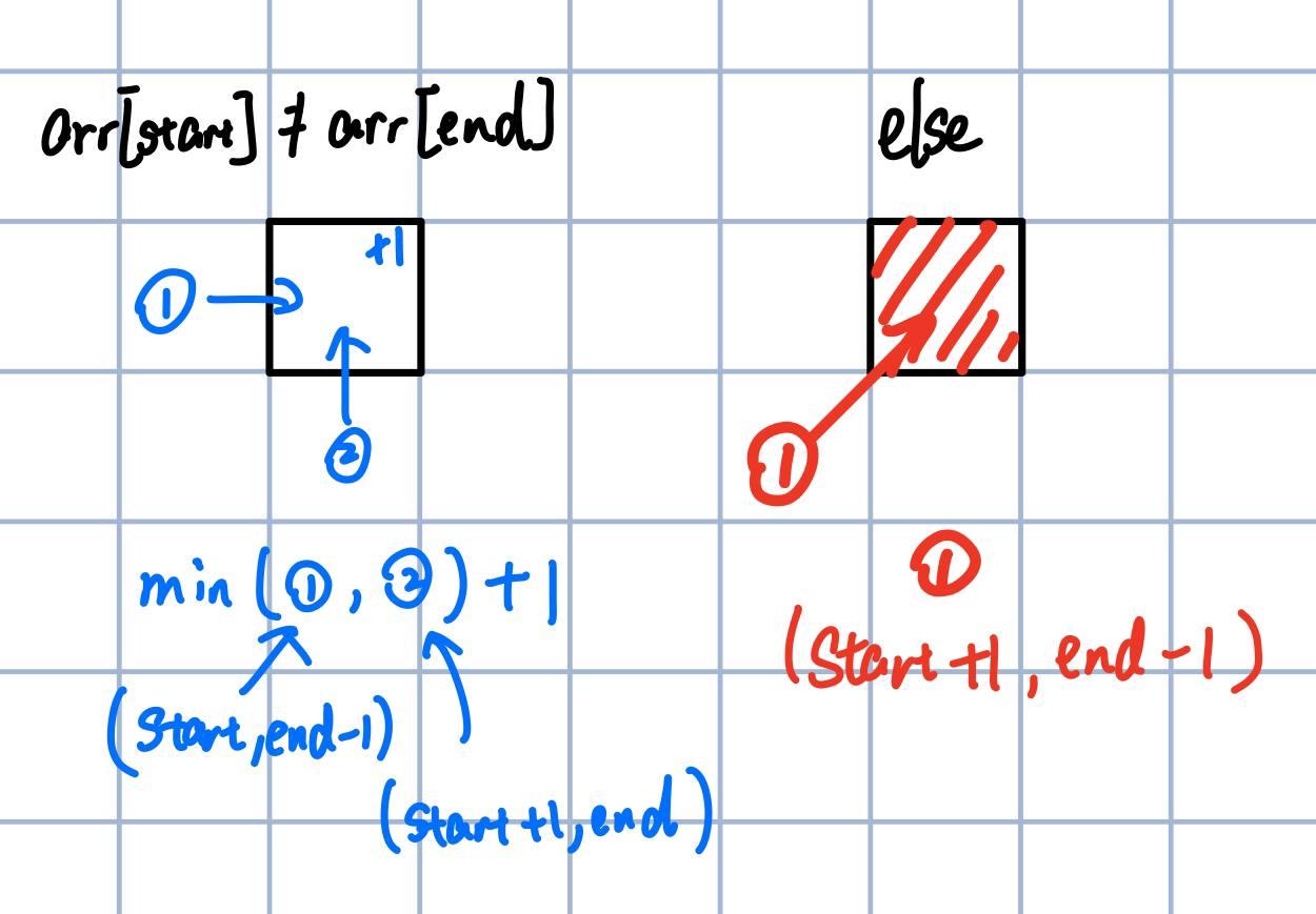
Recalling the analysis, if two characters are equal, it’s like taking a shortcut, which can be observed in this matrix. The figure to the right shows the filling rules for each cell. If characters are equal, directly take the value from the bottom left cell. If they differ, take the minimum value from the left and bottom cells, then add 1.
We can draw a relationship diagram for various grid cells based on the previous graphics:
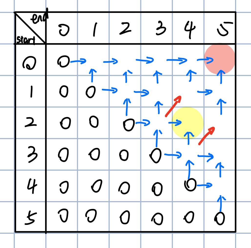
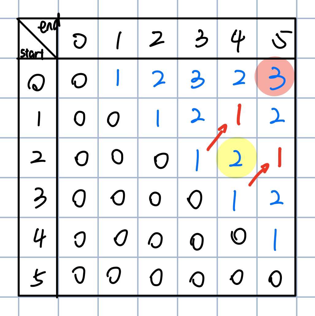
After understanding the relationships, we’re ready to fill in the matrix, yielding the final result of 3.
Here’s the implementation in code:
fn insert_pal_table<T: std::cmp::PartialEq>( arr: &[T] ) -> usize{
    if arr.len() < 2 { return 0; }
    let mut table: Vec<Vec<usize>> = vec![vec![0; arr.len()]; arr.len()];
    for diff in 1..arr.len(){
        let mut i: usize = 0;
        while i + diff < arr.len() {
            if arr[i] == arr[i+diff]{
                table[i][i+diff] = table[i+1][i+diff-1];

            }else{
                table[i][i+diff] = std::cmp::min(table[i][i+diff-1], table[i+1][i+diff]) + 1;
            }
            i += 1;
        }
    }
    return table[0][arr.len()-1];
}
Analyzing this method, we find the time complexity remains O(n^2^), and the space complexity is O(n^2^) - keeping it on par with memory consumption. Still, having a defined table structure offers several optimization opportunities.
Can We Save a Bit More?! - Writing the Algorithm in an Unreadable Way
The reason the previous algorithm had O(n^2^) space complexity was due to storing values in the entire n*n matrix, which may not be necessary. Each value is needed only temporarily and can be discarded once used.
When calculating a box, we only need data from the previous two diagonals. The two diagonals closest to the matrix diagonal contain 2*str.len()-3 items, which is sufficient to cover the maximum memory space needed for future values. Summarily, this is the maximum memory space we require.
Here’s the code implementation:
fn insert_pal_table_mem_opt<T: std::cmp::PartialEq>( arr:&[T] ) -> usize{
    if arr.len() < 2 { return 0; }
    let mut temp: Vec<usize> = vec![0; 2*arr.len() - 3];
    let diff: usize = arr.len();
    for i in 0..arr.len()-1{
        temp[i+arr.len()-2] = 1 - (arr[i] == arr[i+1]) as usize;
    }
    for i in 2..arr.len() {
        for j in 0..arr.len()-i{
            if arr[j] == arr[j+i]{
                temp[ (i%2)*(arr.len()-2) + j ] = temp[ (i%2)*(arr.len()-2) + j + 1];
            }else{
                temp[ (i%2)*(arr.len()-2) + j ] = std::cmp::min(temp[ ((i%2)^1) * (arr.len()-2) + j], temp[ ((i%2)^1) * (arr.len()-2) + j + 1]) + 1;
            }
        }
    }
    return temp[ ((arr.len()-1)%2)*(arr.len()-2) ];
}
Personally, I felt like a warrior when I managed to write this part of the code
With this approach, we achieve an algorithm with space complexity at O(n) level. In terms of time complexity, it’s O(n^2^), but subsequent practical tests confirm that the runtime of O(n^2^) algorithms is faster than the previous one. Using a one-dimensional array makes addressing faster than a two-dimensional one.
After a series of operations, we successfully optimized the original recursive algorithm (O(2^n^) time complexity and O(n) space complexity) into its current form.
Formulating a Dynamic Programming Formula
$F[s,e] = (arr[s]==arr[e]) * F[s+1, e-1] + (arr[s]!=arr[e]) * min(F[s+1, e], F[s, e-1])$
Essentially an
ifoperation: ifarr[s]==arr[e], returnF[s+1,e-1]; otherwise, return themin(...)of the subsequent values
It’s important to note that the derivation of this formula and its usage in code directly stem from the recursive structure. Even without stating what the problem is and just providing the recursive code, it can be completely converted into the form described above. Thus, when practicing coding problems, focus on understanding how the formula is derived and how to apply it.
The reason why I mentioned the recursive part as the most challenging is that figuring out how to break down the problem into smaller subproblems requires trial and error. Once you understand the recursive pattern, the steps to optimize it are fixed. In simple terms, figuring out recursion requires brainpower, while optimizing recursion requires diligent effort.
The formula can be directly translated into code using a strict tabular structure, and this format allows for multiple optimization methods. Hence, when doing coding challenges, reaching the strict tabular structure is usually a good stopping point (assuming you know these optimization techniques). But remember, mastering these optimization tricks is crucial; after all, having a sword and not using it is completely different from not having a sword.
Actual Runtime and Space Analysis
Randomly generating 10,000 strings of fixed length, I tested the execution time of each algorithm (in microseconds) for different string lengths, excluding the dynamic programming recursion due to feasibility.
| 100 Characters (unit: microseconds) | Min | 25th | Med | 75th | Max |
|---|---|---|---|---|---|
insert_pal_map |
68 | 72 | 76 | 94 | 193 |
insert_pal_table |
10 | 10 | 11 | 12 | 26 |
insert_pal_mem_opt |
6 | 6 | 6 | 6 | 14 |
| 1,000 Characters (unit: microseconds) | Min | 25th | Med | 75th | Max |
|---|---|---|---|---|---|
insert_pal_map |
12,167 | 12,671 | 12,775 | 12,909 | 22,592 |
insert_pal_table |
2,535 | 2,707 | 2,817 | 2,923 | 5,036 |
insert_pal_mem_opt |
541 | 554 | 557 | 570 | 1,069 |
| 10,000 Characters (unit: microseconds) | Min | 25th | Med | 75th | Max |
|---|---|---|---|---|---|
insert_pal_map |
1,167,935 | 1,176,727 | 1,187,388 | 1,223,231 | 1,645,885 |
insert_pal_table |
509,278 | 522,494 | 526,456 | 531,771 | 597,337 |
insert_pal_table_mem_opt |
53,285 | 53,705 | 54,543 | 54,835 | 69,375 |
Yes, it took my poor i5 CPU 6 hours to run the 10,000 characters test
100,000 Characters - Only insert_pal_table_mem_opt could handle it without surpassing my 16GB memory, running at approximately 5s per string.
Lastly, I recommend a course on algorithms on Bilibili. I happened to learn these optimization techniques there, and after applying them in practice, this article serves as my personal notes.